1 From Basic Kalman Filter to Complementary Kalman Filter
The Kalman filter has endured since it was invented by Kalman in 1960 and applied to the Apollo moon program, and is now used in robotics, autonomous driving, flight control, and other fields. The basic Kalman filter can only model linear systems; the extended Kalman filter makes a linear approximation to nonlinear equations in order to apply the Kalman filter to nonlinear systems. Later researchers found that separating the system state into major components and errors and using the Kalman filter to predict the errors resulted in a better approximation of the system and better results. In the attitude solving task, researchers used auxiliary sensors such as accelerometers and magnetometers to correct the integration results of the angular velocity meter to obtain a form of complementary Kalman filter. The Kalman filter is a tool, and different ways of modeling the real-world problem result in different forms of the Kalman filter. This leads to the fact that for beginners it is not good to know where to start. It also seems that there are few articles that summarize the basic Kalman filter to various forms of filtering, so this article was created. This article will analyze and explain the various Kalman filter forms from the following aspects.
Basic Kalman filter – prediction for linear systems
Extended Kalman filter – extension of the basic Kalman filter to nonlinear systems
Four-element-based Kalman filter – Explanation based on practical problems
State error Kalman filter – introducing state error into the state vector
Complementary Kalman filter – a form of filter that uses only angular error and angular velocity error as state vectors and measurement vectors
2 Symbol Definition
Lowercase letters are variables; bolded lowercase letters are vectors; uppercase and bolded uppercase are matrices
3 Basic Kalman filter
Macroscopic understanding
Kalman filtering consists of two steps
Prediction (predicTIon) – Dynamic model
Update (correcTIon/measurment update) – ObservaTIon model
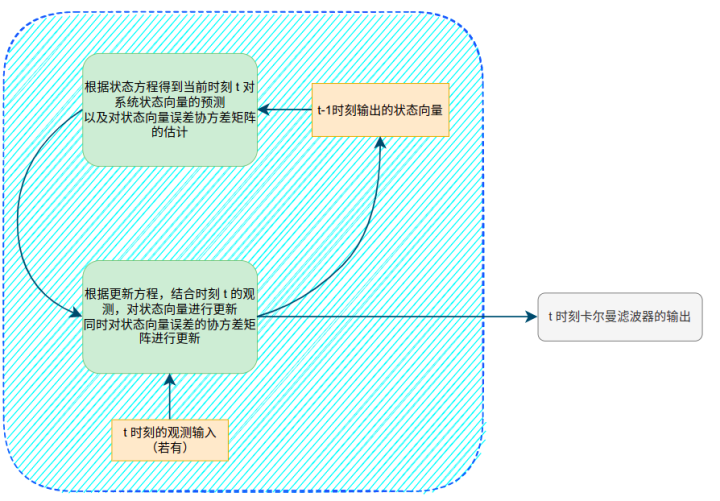
A prediction is a mathematical model that directly calculates the state of the system at this time based on the current sensor input. It can be understood as a calculation of equations. The so-called update is to obtain some other system state input (we call this value measurement value) at some or every moment, compare the predicted system state with the measured system state at this moment, and make a correction to the predicted system state, so it is also called measurement update. The overall framework is shown in the figure below
The state equation and the measurement equation
where is the system state vector and is the measurement vector. are the process noise and observation noise, respectively, and satisfy the Gaussian distribution
The prediction process
where is the error covariance matrix of the a priori state
Update process
Detailed formula derivation

As an overview article, this paper does not carry out the derivation of the basic Kalman filter formula in order not to make it too lengthy. To fully understand the basic Kalman filter, you can refer to the following sources.
Kalman filter basics and formula derivation – a more visual explanation of the probability distribution relationship between the two processes of prediction and update
wiki Kalman Filter – an accurate formulaic derivation
How to understand the Kalman Filter?
From the perspective of probability distributions
The Kalman Filter assumes that the process noise in the change of the system state is Gaussian noise with a mean of zero, so that the state vector also becomes a random vector with a Gaussian distribution. Also the noise of the observed process is assumed to be Gaussian noise with mean value 0. The function that maps the state vector to the measurement vector is obtained by the measurement equation, i.e., Equation (1-2). Thus, when the measurement values are obtained, an additional estimate of the state vector can be derived using the relationship between the measurement values and the state vector. Both the state estimate and the state equation calculated using the measurement values conform to the Gaussian distribution, and the joint probability distribution of the two Gaussian distributions still maintains the Gaussian property. Further derivation leads to Eqs. (1-5) to (1-7). For an understanding of this perspective you can read the first article recommended above.
From the perspective of minimizing the error
The final output of the Kalman filter is that the true state is such that the square of the error is minimized, and again Eqs. (1-5) to Eqs. (1-7) can be deduced. Thus the Kalman filter is also an optimal estimate of the system state. For the understanding and derivation of this perspective, you can refer to the second article recommended above.
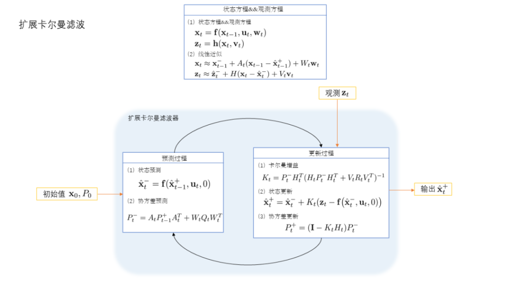
4 Extended Kalman filter
Linear approximation of nonlinear equations
The Kalman filter is built on the linear state and measurement equations also known as Equation (1-1) and Equation (1-2). However, in practical applications, more relationships are non-linear, such as how to calculate the current attitude angle of the vehicle from the continuous angular velocity, etc. To be able to utilize the prediction and update process of the basic Kalman filter, for the nonlinear state and observation equations, we approximate the nonlinear formulas as linear formulas using a first-order Taylor expansion.
7b160e28-7c18-11ed-8abf-dac502259ad0.png
Equation of state and measurement equation
Equations (2-1, 2-2) can be analogous to equations (1-1, 1-2) in the basic Kalman filter
First-order Taylor expansion
We first assume that the output of the filter at the known moment, that is, the state posterior at the moment, and the corresponding covariance matrix is At the same time, we make the prior to do an expansion of Eq. (2-1) at this point and keep only one term At the same time, do a Taylor expansion of Eq. (2-2) at this point and keep only one term In Eqs. (2-4) and (2-5).
The prediction equation and the state covariance matrix
where the second term in Eq. (2-7), because in the linear approximation equation (2-4), the noise term satisfies the distribution
Updating the equations and Kalman gain
5 Basic Kalman filter && Extended Kalman filter summary

6 Expanded Kalman filter based on quaternions
Starting from a practical problem
In the attitude estimation of moving objects, such as the attitude calculation of vehicles, the IMU (InerTIal Meseasurment Unit) inertial measurement unit is often used to calculate the attitude of the object. For the sake of description, attitude estimation here means that we want to solve for the deflection angles of the three axes between the vehicle and the starting coordinate system at each moment, usually denoted by roll, pitch, and yaw.
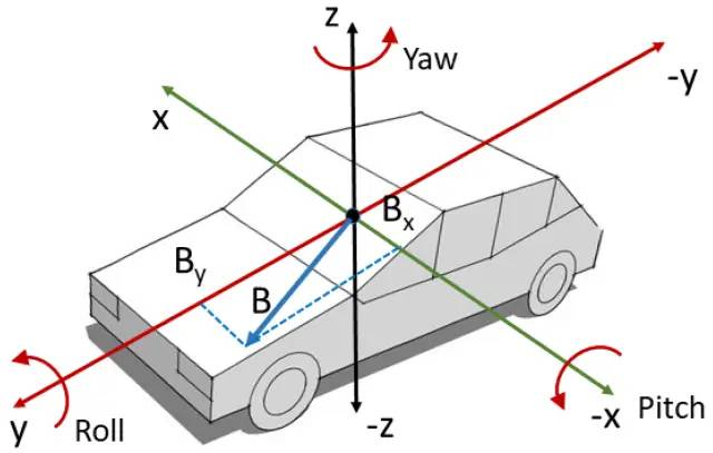

IMU (Inertial Measurement Unit)
Nowadays, IMUs are generally six-axis or nine-axis. Six-axis IMU can output acceleration (acc) and angular velocity (gyro) of three axes; while nine-axis adds Magnetometer (magnetometer) to six-axis to measure magnetic field direction of three axes. To simplify the problem, we use the six-axis IMU as an example.
Related Definitions
In various fields of attitude estimation, a quaternion is commonly used to represent a rotation. The quaternion has better properties than the Euler angular expression and is more compact compared to the rotation matrix. The quaternion is defined as follows To estimate the attitude of the system, it is common practice to track the angular velocity using the inertial measurement unit IMU, whose angular velocity at each moment is defined as In addition, we need to know the output frequency of the IMU. Suppose the output time interval of the IMU is
The derivative of the product of the four elements
This part is prepared for later derivation of the Jacobian matrix in the equation of state of the extended Kalman filter We let the rotation of the moment be . The rotation of the moment is. Then the rotation of the moment is obtained by the change of the rotation of the moment through which is equal to the amount of angular change in the time interval. In a very short time interval, we consider the change in angle to be uniform, i.e. We let the rotation axis of the angle in this time interval is and the rotation angle is,then According to the basic knowledge of quaternion, we can get One of the key points of the extended Kalman filter is to find the partial derivative of the state equation with respect to the state; although we can derive the discrete form of the angle integral from the output of the triaxial angular velocity (1), we can’t actually find the partial derivative of it directly. As to why we cannot derive the derivative directly, the following is a good point:
The definition of derivative is the limit of the micro-increment of the function value with respect to the micro-increment of the independent variable. After the unit quaternion of the rotation has been differentiated, it is no longer a unit quaternion, and is not a rotated quaternion
In order to be able to find the partial derivative of Eq. (1), we first find the derivative of the rotation with respect to time. Then, using Taylor expansion, we expand Eq. (1) as a linear equation and take only one term, so that we can obtain We have the derivative of the angle with respect to time, we can expand Eq. (1) using Taylor expansion and keep only one term, then we can obtain
State vector and control input
We directly express the attitude angle of the vehicle in quaternion form as the system state vector and the three-axis angular velocity of the IMU at each moment as the control input
State equation and its Jacobi matrix
With the derivation of the previous section on the four-element derivatives, we can directly write the state equation as follows where is the random noise with a covariance matrix of
Prediction equation
Since the Jacobian matrix has been derived in the above derivation, the prediction equation can be written directly according to the extended Kalman filter formula
Measurement update
In the previous section, we used the angular velocity meter output as the control input and constructed the state and prediction equations. IMUs typically have accelerometer outputs, which can be used as measurement quantities and to perform measurement updates to the predicted state. We first review the process of updating the state vector in the measurement update. Let the accelerometer output be the measurement vector.
Measurement model
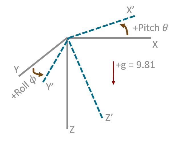
Now that we have identified the state vector as the quaternion expression of the attitude angle and the measurement vector as the output of the accelerometer in all three axes, what form is the function going to take that will convert the attitude angle to a three-axis acceleration? The key connection is that when the vehicle is at rest, the combined vector of acceleration is the acceleration of gravity, vertically downward!

In the figure above, the coordinate system is assumed to be the starting coordinate system, which is the coordinate system after the cart is moved. At the start, the trolley is stationary and the output of the gravitational acceleration of the trolley is vertical downward, i.e. We use the normalized form, which means that the gravitational acceleration is treated as one unit. Then, when the car is moving, the expression of the acceleration of gravity in the coordinate system is and is the expression of the acceleration of gravity in two different coordinate systems, while the rotation between these two coordinate systems is the state vector at this time, so where is the expression of converting the quaternion into a rotation matrix, and the left multiplication of the rotation matrix by a three-dimensional column vector indicates a three-dimensional rotation of this vector. That is, the following form (which is what we defined before)
Jacobi matrix
From equations (3-7) we can obtain the Jacobian matrix of the transformation function in the measurement model
Updating the equations
7 State Error Kalman Filter (ErKF : Error-state Kalman Filter)
Overview
In using Kalman filter for Attitude Estimation, a large part of the system attitude angle is not directly used as the state of the Kalman filter, but the integration error of the attitude angle and the error of the angular velocity meter are used as the system state. The output of the angular velocity meter is used to compensate for the estimated angular velocity meter error, and then it is integrated to obtain an estimate of the attitude angle, and then the error estimate of the attitude angle is compensated for. The entire flow chart is shown in the following diagram, which is quoted from Intertial Head-Tracker Sensor Fusion by a Complementary Separate-Bias Kalman Filter

PS: It is important to emphasize that there are various forms of Kalman filter, and the definitions of various symbols are not exactly the same, which is also a difficult place to get started with Kalman filter. This is also the purpose of this article, to provide a basic overview to the beginners of Kalman filtering. Therefore, the ErKF given here is just one of the forms, mainly quoted from the paper Extended Kalman Filter vs.
Recursive formulation of the state error
First, we make the state vector represent the time-continuous form. The derivative with respect to time is added to the right-hand side of the equal sign as a small perturbation, and the function is expanded according to the Taylor expansion. The above equation is then expressed in discrete form, i.e. With the recursive formulation of the state error, we can derive the prediction and update process as in the Kalman filter
Prediction process
Slightly different from doing the Kalman filter directly on the system state, the Kalman filter using the error state can be seen as three steps when calculating the attitude angle.
Calculate the system state at this point using integration outside the Kalman filter system
Use Kalman filter to calculate the error of the system state at this time
Integrate the system state to compensate for the Kalman filter error
System state calculation
The above equation is just a formulaic expression, which is actually the state of the previous moment, plus the amount of change of the state in this time period. In attitude estimation, the amount of state change is usually the output of the angular velocity meter multiplied by the time interval.
State error equation and prediction equation
The equation of state error can be obtained from Equation (4-1) where is the process noise and the covariance matrix is the prediction equation Similar to the ordinary Kalman filter, the prediction equation is
Measurement equation and update equation
Here we directly use the attitude calculated using the rest of the sensors such as accelerometer and magnetometer as the measurement quantity of the system. Remember here first that the accelerometer can calculate the angle based on the output pinch angle, and by the magnetometer can just calculate the angle. Of course, other sensors that can directly output the system attitude angle can be used as the measurement value. The measurement equation where is the measurement noise and the covariance matrix is Update the equation Here two update steps are performed
First, the estimate of the state error is updated
Update the estimate of the state (i.e., make up the state error to)
Supplementary
In the above derivation, our target variable, the attitude angle of the system, is computed as a separate integral outside, but it is actually more common to compute the deviations of attitude angle and angular velocity directly in the state vector. The angular velocity deviation at each moment is then applied to the output of the angular velocity meter, which is then applied to the state equation as a system input. That is, like the illustration in the overview. But in fact the various Kalman filters are modeled differently, and the Error-state Kalman Filter and Complimentarty Kalman Filter are not strictly defined. So simply this section is treated as an understanding and derivation of the state errors, and a Kalman filter that seems to be more widely used is given in the following complementary Kalman filter.
8 Complementary Kalman Filter
Preface
As mentioned earlier, Kalman filters have been modeled in various forms and many studies have been done in the last century. There is actually no strict definition for the Error-state Kalman Filter and the Complementary Kalman Filter. The Comlimentary Kalman Filter here can actually be seen as another form of the ErKF above. There is so much work on Kalman filtering, and so many blogs and papers, that it seems very difficult. This paper looks good in terms of citations, paper narrative, and symbol identification, and is a good read for engineers who want to apply Kalman filtering to pose estimation. There is even some work that uses the normal Kalman filter output directly and then uses the concept of complementary filters to do weighted averaging between multiple pose outputs, also called complementary Kalman filters, such as this patent: A method for computing fused pose angles based on the complementary Kalman filter algorithm
The concept of complementarity
In fact, as long as the angular velocity meter (Gyroscope) is available we can solve the attitude angle of the vehicle based on its output and do the integration in time. However, since any sensor is noisy, at the same time, the error will accumulate randomly over time when solving directly by integration, and the final attitude solution accuracy will be very poor. In addition to the integration using angular velocity meter to obtain the attitude angle, the attitude of the dynamic system can also be calculated using Accelerometer and Magnatometer. Among them, the accelerometer uses the acceleration of gravity as the anchor quantity and measures the angle between the acceleration of the three axes at rest to calculate the angle; the magnetometer (or geomagnetometer) uses the north pole of the Earth’s magnetic field as the anchor quantity to calculate the angle. Using these two to complement the angular velocity meter yields a more accurate attitude estimate.
Calculating attitude angle roll, pitch from accelerometer
The Accelerometer can output the acceleration of three axes, and in the stationary case, the combined vector of the three axes is the gravitational acceleration. Therefore, we can use the relationship between the acceleration of the three axes to calculate the pitch and roll angles at rest
For more information on how to derive the roll and pitch from the acceleration of the three axes, see this article The final form is also very simple.
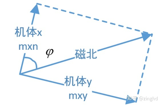
Calculating the attitude angle yaw from the magnetometer
The three-axis merging vector of the magnetometer will point to the geomagnetic north pole, and using this property, the angle of deflection from the output of the magnetometer to the geomagnetic north pole can be obtained. Using this, the angle relative to the starting position can be calculated
The specific calculation formula can be found in this blog
Attitude compensation from acceleration calculation
The roll and pitch angles can be calculated from the accelerometer, so this result can be combined with the integral result of the angular velocity to get a better estimate of the attitude. However, it is important to note that there are two limitations of attitude compensation from acceleration.
The accelerometer can only calculate the Roll and Pitch angles, so complementary information is not available for the yaw angle
When the vehicle is in a larger acceleration motion, the combined vector of the three axes acceleration will deviate from the gravitational acceleration, so the complementary results should be changed according to the magnitude of this deviation.
Complementary filter
The complementary filter uses the integration result of the angular velocity and the calculation result of the acceleration and magnetometer to interpolate and get a better result Where is the attitude (expressed in four elements) obtained by integrating the angular velocity; is the attitude calculated using the accelerometer and magnetometer.
Complementary Kalman filter
The complementary Kalman filter treats the error in the attitude angle, and the error in the angular velocity as state vectors; and uses the difference between the attitude angle calculated by the remaining sensors, such as accelerometers and magnetometers, and the estimated attitude angle as the measured quantity. The attitude angle of the system is obtained by the following steps.
The Kalman filter outputs the error of the attitude angle and the error of the angular velocity
Add the output of the angular velocity at the current moment to the error of the angular velocity and use the integral formula to calculate the attitude angle
Add the attitude angle calculated in step 2 to the attitude angle error output in step 1
State vector and measurement vector
State vector where is the angle of the system; is the three-axis angular velocity. Measurement vector where is the angle of the system calculated using accelerometers and magnetometers
Equation of state
We can derive the derivative of the attitude angle with respect to time, which is usually a function of the attitude angle and the angular velocity, i.e. From the derivation of Eq. (4-1) and the Taylor expansion, we can obtain the recursive equation We directly assume that the error of the angular velocity is a constant error, i.e. Then we can write the above two equations in matrix form
Measurement equation
Prediction && update process
With the derivation of the state equation and the measurement equation above, all that remains is to follow the process of substitution from equation (4-3) to equation (4-10). The only difference here is that the Kalman filter output vector is the error of angular velocity and the error of attitude. When calculating the attitude first apply the error of angular velocity to the angular velocity meter data, integrate the angle, apply the error of angle to the angle integration result, and get the final angle output. The whole framework is shown below

9 Postscript
Kalman filtering is a very old algorithm, but at the same time it is widely used. Even though many factor maps are used in today’s attitude solving, the pre-integration of IMUs still uses Kalman filtering. However, the Kalman filter algorithm is just a tool, and different ways of modeling the system will produce different forms of Kalman filters, which leads to beginners not knowing where to start.
In the process of checking information, I found that some variants of Kalman filter such as Error-State Kalman Filter and Complimentary Kalman Filter are actually not strictly defined.
The author does not have rich experience in Kalman filter applications, nor does he specialize in motion control and attitude solving. In this paper, I have tried my best to ensure the accuracy of the formulas and symbol definitions in addition to the pursuit of easy understanding. However, there is no guarantee that there are no errors.
The initial value setting of each variable in the Kalman filter is a matter of study, and there is a separate section in the paper on how to set the initial value. This may have to be combined with practical applications and results to arrive at the optimal solution.
10Reference
[1] Roll and Pitch Angles From Accelerometer Sensors [2] Quadratic, Eulerian, and Rotation Matrix Conversions [3] Four-Element Product Derivation [4] A Complementary Kalman Filter Algorithm-Based Method for Calculating Fused Attitude Angles [5] Inertial head-tracker sensor fusion by a complementary separate-bias Kalman filter [6] Extended Kalman Filter vs. Error State Kalman Filter for Aircraft Attitude Estimation [7] Original Paper on Kalman Filter [8] Kalman Filter Basics and Formula Derivation